Purpose
Use this statement to retrieve data from tables or views.
Prerequisites
-
You need either the system privilege
USE ANY SCHEMAor the object privilegeUSAGEon the target schema, or the schema must be owned by you or one of your assigned roles. - You need either the system privilege
SELECT ANY TABLEor theSELECTobject privilege on tables or views which are referenced in theSELECTlist, or the tables or views must be owned by you or one of your assigned roles. - When accessing views, the owner of the view must have
SELECTprivileges on the objects that are referenced in the view. - If you use a subimport, you need the appropriate rights similar to the IMPORT statement.
Syntax
subquery::=


with_clause::=

select_list::=
from_item::=
connect_by_clause::=

preferring_clause::=

preference_term::=
group_by_clause::=
cube_rollup_clause::=

grouping_sets_clause::=

grouping_expression_list::=
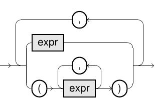
order_by_clause::=

limit_clause::=

join_clause::=

inner_outer_clause::=

subimport::=

values_table::=
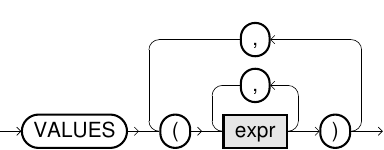
value_range_table::=

Usage notes
-
You can calculate scalar expressions by omitting the
FROMclause. For example:SELECT 'abc'. -
You can use the
WITHclause to define common table expressions (CTEs). These are temporary views that are valid only during the execution of a subquery. -
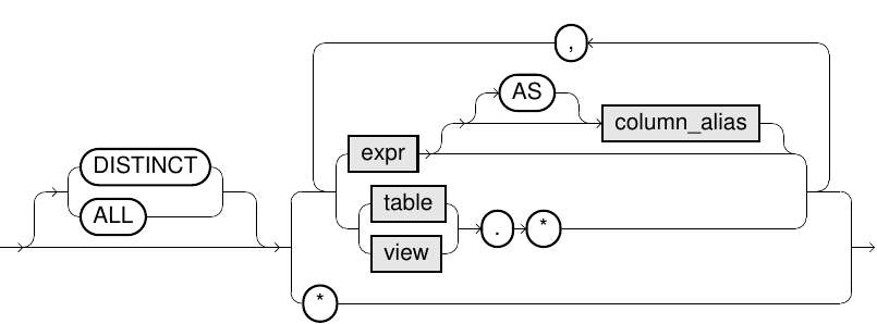
To eliminate identical rows, use
DISTINCT. If you use the keywordALL(default), all rows will be present in the result table. -
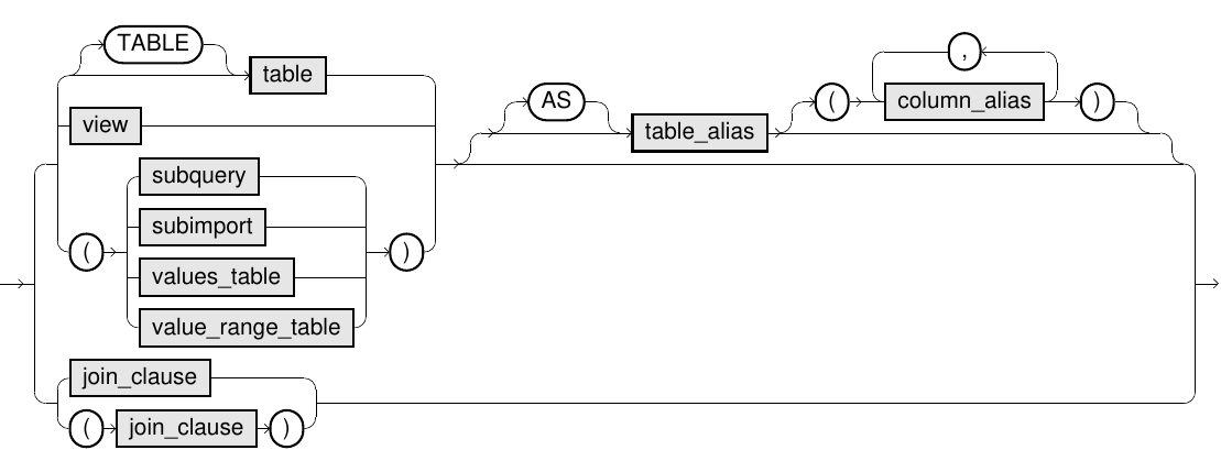
To define the source tables or views, use the
FROMclause. You can define static tables in avalues_table. For example,(VALUES (1, TRUE), (2, FALSE), (3, NULL)) AS t(i, b)defines a table with two columns and three rows. -
The
select_listdefines the columns of the result table. If*is used, all columns are listed. You can use an expression liket.*to list all columns of the tablet
, the viewt
, or the object with the table aliast
. -
If you have complex expressions within a
select_list, consider using column aliases. You can only reference such aliases directly inside theORDER BYclause and theQUALIFYfilter condition. However, you can also reference those aliases indirectly through the keywordLOCALwithin the other clauses (WHERE, GROUP BY, HAVING), and even in theSELECTlist. Column aliases define the column names of the result table.Example of indirect referencing:
SELECT ABS(x) AS x FROM t WHERE local.x>10 -
Unqualified column names (without a table prefix) are resolved to table columns from the
FROMclause, except inORDER BYandQUALIFY, whereselect_listnames are preferred over table columns. To resolve ambiguity and improve readability, use table name or alias when referring to table columns, andLOCALwhen referring toselect_listnames. -
To restrict the result by certain filter conditions, you can use the
WHEREclause.You can specify equality join conditions among tables within the
WHEREclause by using the=operator. If you want to define an outer condition, add(+)after the outer expression. -
The
CONNECT BYclause can be used to define hierarchical conditions. This clause is evaluated before theWHEREconditions, excepting the join conditions on tables that are referenced in theCONNECT BYclause itself.
The following elements are relevant for theCONNECT BYclause: -
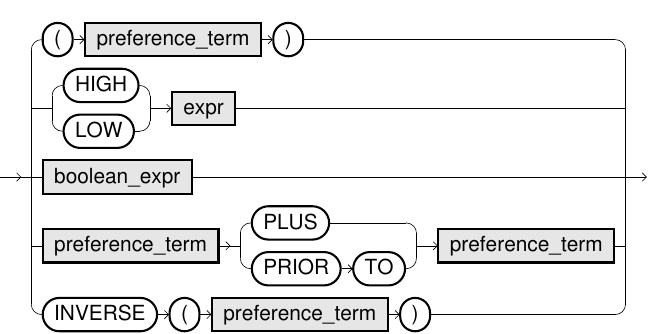
The
PREFERRINGclause defines a Skyline preference term. For more information, see Skyline. -
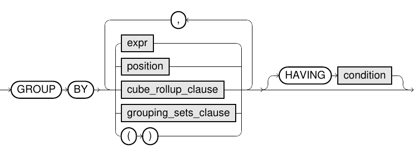
The
GROUP BYclause defines groups of rows which will be aggregated in the result table. You can use aggregate functions in theselect_list. Using a numerical value n (position) results in aggregating the result table by the nth column. For example,GROUP BY1is equivalent toGROUP BYthe first column inselect_list.If
GROUP BYis used, allSELECTselect_listelements must be aggregated except those that define the grouping keys. -
CUBE,ROLLUP, andGROUPING SETSare extensions of theGROUP BYclause for calculating superaggregates. These are hierarchical aggregation levels, such as partial sums for days, months and years, and can be computed within one singleGROUP BYstatement instead of using aUNIONof several temporary results.You can distinguish between regular result rows (normal aggregation on the deepest level) and superaggregate rows. The total of all arguments results in the normal aggregation, and the subsets result in the corresponding superaggregates. You can discern the result row types by using the function GROUPING[_ID].
-
To restrict the result by filter conditions that contain or reference analytic functions, use the
QUALIFYclause.If the condition does not contain an analytic function, use the
WHEREorHAVINGclauses, since the filter forQUALIFYis evaluated later. -
To sort the result table, use the
ORDER BYclause.-
Using a numerical value n (position) results in sorting the result table by the nth column, for example,
ORDER BY1. -
String data is sorted by its binary representation.
-
Options for the
ORDER BYclause:ASCmeans ascending order,DESCmeans descending order. If not specified, results are sorted in ascending order.NULLS LASTandNULLS FIRSTdetermine ifNULLvalues are sorted at the end or the beginning of the result list. If not specified,NULLresults will be at the end of the result list.
-
-
To restrict the number of result rows you can use the
LIMITclause.-
The optional offset can only be used in combination with
ORDER BY. -
LIMITis not allowed within correlated subqueries. -
LIMITwithOFFSETis not allowed in aggregatedSELECTstatements withoutGROUP BY.
-
-
To integrate the import of external data sources directly in your query, you can use the
subimportclause.-
For information about the usage of external data sources and their options, see IMPORT.
We strongly recommend that you explicitly specify the target column types when importing data from external sources. Otherwise, the column names and data types are chosen in a generic way. For importing files, these types are mandatory.
-
Local files cannot be imported directly within queries.
-
By creating a view, external data sources can be integrated with Exasol as a sort of external tables.
-
Local filter conditions on such imports are not propagated to the source databases. However, you can achieve that by using the
STATEMENToption.
-
-
SELECTstatements can be combined using the table operatorsUNION ALL,UNION,INTERSECT, andMINUS (=EXCEPT). For more information, see Table Operators - UNION [ALL], INTERSECT, MINUS. -
The arguments
min_valueandmax_valuein theVALUES BETWEENclause must be constant expressions that evaluate to integers. The argumentstep_valuemust be a constant expression that evaluates to a positive integer.The value range table has a single column with the name
RANGE_VALUEand an integer type (DECIMAL(9,0),DECIMAL(18,0), orDECIMAL(36,0)as appropriate). The column contains all the values betweenmin_valueandmax_valuecombined if no step is given. If a step is given, the column skips values and produces the arithmetic seriesmin_value + step_value * nwith the last value less than or equal tomax_value. See also Example 7.VALUES BETWEENis significantly faster than usingCONNECT BYto generate a range of values. -
The
WINDOWclause allows the definition of named window specifications (i.e. the content ofOVERclauses) for analytic functions. For more information, see Analytic functions. -
The query cache stores a
SELECTquery together with its result if certain conditions are fulfilled. If the same query is sent again, the database can read the result directly out of the cache instead of executing the query. For more information, see ALTER SYSTEM.
| Elements | Meaning |
|---|---|
START WITH
|
Specifies the set of root nodes in the graph. |
condition(s)
|
You can define multiple conditions. A hierarchical connection between parent and child rows can be defined by the keyword PRIOR (for example, PRIOR employee_id = manager_id). If you do not specify such a PRIOR condition, the cross product will be computed. Thus, the statement SELECT LEVEL FROM dual CONNECT BY LEVEL<=100 results in a table with 100 rows, because 100 cross products were calculated for the table dual. |
NOCYCLE
|
If you specify this option, the query also returns results if a cycle exists. In this case the expansion will be terminated when a cycle is detected. |
The following functions and operators can be used in the select_list and in the WHERE conditions to qualify the results of a hierarchical query.
| Functions and operators | Meaning |
|---|---|
SYS_CONNECT_BY_PATH (expr,
char)
|
Returns a string containing the full path from the root node to the current
node, containing the values for expr and separated by char. |
LEVEL
|
Returns the hierarchy level of a row: 1 for the root node, 2 for its direct children, and so on. IMPORTANT: Cycle detection is disabled if |
PRIOR
|
This operator references the row’s parent row, which allows you to define a parent-child condition. You can also use this operator to access the values
of the parent row. Hence, the following two
|
CONNECT_BY_ROOT
|
Instead of a row’s value, the corresponding value of the root node is used. For example, |
CONNECT_BY_ISLEAF
|
This expression returns 1 if a row is a leaf in the tree (the row has no
children), otherwise 0. |
CONNECT_BY_ISCYCLE
|
Returns whether the current row causes a cycle. In the path, such a row will occur exactly twice. This expression can only be used in combination with the NOTE: This behavior is different to Oracle’s implementation, where the parent node is returned instead of the connection point of the cycle. |
The function LEVEL and the operator PRIOR can also be used within the CONNECT
BY clause.
| Grouping | Meaning |
|---|---|
CUBE
|
Calculates the aggregation levels for all possible combinations of the arguments (2n combinations). Example: By |
ROLLUP
|
Calculates the aggregation levels for the first n, n-1, n-2, ... 0 arguments (overall n+1 combinations). The last level corresponds to the grand total. Example: By This expression is equivalent to |
GROUPING SETS
|
Calculates the aggregation levels for the specified combinations. CUBE and ROLLUP are special forms of GROUPING SETS and simplify the notation. |
()
|
Is similar to GROUPING SETS () and aggregates the whole table as one single group. |
If multiple hierarchical groupings are specified as a comma-separated list, the result is the set of all combinations of partial groupings (cross product). For example, the expression ROLLUP(a,b),ROLLUP(x,y) results in 9 combinations. Starting with the subsets (a,b), (a), () and (x,y), (x), () you get the following combinations: (a,b,x,y), (a,b,x), (a,b), (a,x,y), (a,x), (a), (x,y), (x),().
To restrict the number of groups, you can use the HAVING clause.
Examples
Customers table
SELECT * FROM customers;| C-ID | NAME |
|---|---|
| 1 | smith |
| 2 | jackson |
Sales table
SELECT * FROM sales;| S-ID | C_ID | PRICE | STORE |
|---|---|---|---|
| 1 | 1 | 199.99 | MUNICH |
| 2 | 1 | 9.99 | TOKYO |
| 3 | 2 | 50.00 | MUNICH |
| 4 | 1 | 643.59 | TOKYO |
| 5 | 2 | 2.99 | MUNICH |
| 6 | 2 | 1516.78 | NEW YORK |
The following examples relate to the customers and sales tables above:
Example 1
SELECT store, SUM(price) AS volume FROM sales
GROUP BY store ORDER BY store DESC;| STORE | VOLUME |
|---|---|
| TOKYO | 653.58 |
| NEW YORK | 1516.78 |
| MUNICH | 252.98 |
Example 2
SELECT name, SUM(price) AS volume FROM
customers JOIN sales USING (c_id)
GROUP BY name ORDER BY name;| NAME | VOLUME |
|---|---|
| jackson | 1569.77 |
| smith | 853.57 |
Example 3
WITH tmp_view AS (SELECT name, price, store FROM customers, sales
WHERE customers.c_id=sales.c_id)
SELECT sum(price) AS volume, name, store FROM tmp_view
GROUP BY GROUPING SETS (name,store,());| VOLUME | NAME | STORE |
|---|---|---|
| 1569.77 | jackson | |
| 853.57 | smith | |
| 653.58 | TOKYO | |
| 252.98 | MUNICH | |
| 1516.78 | NEW YORK | |
| 2423.34 |
Example 4
SELECT * FROM (IMPORT INTO (v VARCHAR(1))
FROM EXA AT my_connection
TABLE sys.dual);SELECT last_name, employee_id id, manager_id mgr_id,
CONNECT_BY_ISLEAF leaf, LEVEL,
LPAD(' ', 2*LEVEL-1)||SYS_CONNECT_BY_PATH(last_name, '/') "PATH"
FROM employees
CONNECT BY PRIOR employee_id = manager_id
START WITH last_name = 'Clark'
ORDER BY employee_id;| LAST_NAME | ID | MGR_ID | LEAF | LEVEL | PATH |
|---|---|---|---|---|---|
| Clark | 10 | 9 | 0 | 1 | /Clark |
| Sandler | 11 | 10 | 1 | 2 | /Clark/Sandler |
| Smith | 12 | 10 | 0 | 2 | /Clark/Smith |
| Jackson | 13 | 10 | 0 | 2 | /Clark/Jackson |
| Taylor | 14 | 10 | 1 | 2 | /Clark/Taylor |
| Brown | 15 | 12 | 1 | 3 | /Clark/Smith/Brown |
| Jones | 16 | 12 | 1 | 3 | /Clark/Smith/Jones |
| Popp | 17 | 12 | 1 | 3 | /Clark/Smith/Popp |
| Williams | 18 | 13 | 1 | 3 | /Clark/Jackson/Williams |
| Johnson | 19 | 13 | 1 | 3 | /Clark/Jackson/Johnson |
Example 5
-- Get the largest sale per customer
SELECT S_ID, C_ID, PRICE, ROW_NUMBER() OVER (PARTITION BY C_ID ORDER BY PRICE DESC) NUM FROM SALES QUALIFY NUM = 1;| S-ID | C_ID | PRICE | NUM |
|---|---|---|---|
| 4 | 1 | 643.59 | 1 |
| 6 | 2 | 1516.78 | 1 |
Example 6
-- It is also possible to specify the analytic function call directly in the qualify expression

SELECT S_ID, C_ID, PRICE FROM SALES QUALIFY ROW_NUMBER() OVER (PARTITION BY C_ID ORDER BY PRICE DESC) = 1;| S-ID | C_ID | PRICE |
|---|---|---|
| 4 | 1 | 643.59 |
| 6 | 2 | 1516.78 |
Example 7
SELECT * FROM VALUES BETWEEN 1 AND 15 WITH STEP 4;| RANGE_VALUE |
|---|
| 1 |
| 5 |
| 9 |
| 13 |
Example 8
SELECT v,
       DATE'2020-10-26' + v * INTERVAL'7'DAY AS late_2020_mondays,
       5 * v AS five_times_table
FROM VALUES BETWEEN 1 AND 9 AS v(v);| V | LATE_2020_MONDAYS | FIVE_TIMES_TABLE |
|---|---|---|
| 1 | 2020-11-02 | 5 |
|
2 |
2020-11-09 | 10 |
| 3 | 2020-11-16 | 15 |
| 4 | 2020-11-23 | 20 |
| 5 | 2020-11-30 | 25 |
| 6 | 2020-12-07 | 30 |
| 7 | 2020-12-14 | 35 |
| 8 | 2020-12-21 | 40 |
| 9 | 2020-12-28 | 45 |
