In this tutorial you will learn how to train a data model locally in R and then predict in Exasol using a UDF.
Prerequisites
-
A running Exasol database
-
R development environment such as RStudio
Load data and train in R
Load libraries in R
This tutorial uses data from the BostonHousing
sample data set in the mlbench library.
Also load the libraries RODBC, exasol, randomForest, and RCurl, which will be required in this tutorial.
# load libraries
library(mlbench)         # Load data
library(RODBC)           # ODBC database connectivity
library(exasol)          # R interface for Exasol database
library(randomForest)    # Random forests for regression and classification
library(RCurl)           # HTTP communication
Load data and split into training and testing sets
Load the data into R, then split it into a training set and a testing set. The ratio of the split is arbitrary and depends on the available data and application, but in this case you will keep 75% of the data for training and use the remaining 25% for testing purposes.
There are several methods that you can use to split the data. In this tutorial we use a method that randomly generates indexes that subset rows from the main data set.
# Load data
data("BostonHousing")

# Generate random indices (75% of the sample size)
set.seed(42)
indices <- sample(nrow(BostonHousing),size=floor(nrow(BostonHousing) * 0.75))

# Add a dummy variable with 2 levels "Train" and "Test"
BostonHousing$split = factor(NA, levels = c("Train", "Test"))

# Assign predefined rows respectively to "Train" and "Test" subsets
BostonHousing$split[indices]  = "Train"
BostonHousing$split[-indices] = "Test"

# Add id variable
BostonHousing$id = seq(1:nrow(BostonHousing))
Train the model
You can now train a basic random forest model on our data and see which variables contribute the most to predicting the median house value.
set.seed(42)
# Run model (note that we filter only for the training data (split=="Train"))
rf_model = randomForest(medv ~ .-split -id,
                        data = BostonHousing[BostonHousing$split=="Train",],
                        importance = TRUE)

# See which variables are important in predicting house prices
varImpPlot(rf_model)
# rm    - number of rooms per house
# lstat - % lower status of the population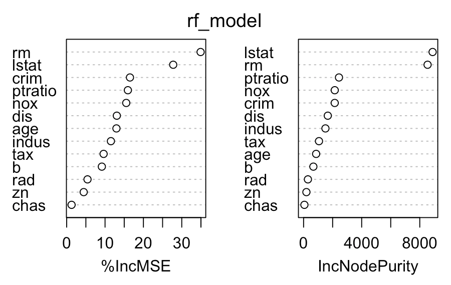
Upload the model to BucketFS
UDF scripts are executed in parallel on the Exasol cluster. The UDF that you will use for prediction must have access to the model that you just trained. You can store the model on any file service, but for performance reasons we recommend that you upload it to BucketFS on the cluster nodes.
BucketFS is a synchronous file system available on all database nodes in an Exasol cluster. You can upload files to BucketFS in R using packages that allow HTTP communication, such as httr or RCurl. In this tutorial you will use the RCurl package to upload the trained model.
The model that lives in the R environment has to be serialized (converted into raw text) when it is uploaded to BucketFS. When it is retrieved from BucketFS it must be unserialized and returned to its original file type.
To learn more about serialization in R, enter ?serialize in RStudio.
For more information about BucketFS, see BucketFS.
Values in angle brackets such as <bucket_name> are placeholders. Replace these with your own values.
# Define options for the authentication
curl_opts = curlOptions(userpwd  = "w:<write_passwd>",
                        verbose  = FALSE,
                        httpauth = AUTH_BASIC)

# Transfer model to the bucket
httpPUT(
  # EXABucket URL (change for your environment)
  url = "http://<Exasol server>:<BucketFS service port>/<Bucket name>/rf_model",
  # It is important to serialize the model
  content = serialize(rf_model, ascii = FALSE, connection = NULL),
  # EXABucket: authenticate
  curl = getCurlHandle(.opts = curl_opts)
)
Load data into Exasol
Load the data into the Exasol database by opening a connection and using the exa.writeData function in the Exasol R package.
To know more about how to write data into an Exasol database from R, see Write data.
# Create connection with the Exasol database
exaconn <- dbConnect(
    drv     = "exa",                  # EXAdriver object
    exahost = "192.168.56.103:8563",  # IP of database cluster
    uid     = "sys",                  # Username
    pwd     = "exasol")               # Password

# Create database schema (if it does not yet exist) with the name r_demo
# (This also opens it, i.e. makes it the default container for all subsequent steps below)
odbcQuery(exaconn, "CREATE SCHEMA IF NOT EXISTS r_demo")

# If the schema already existed, we need to open it to make it the default container for all subsequent steps below
odbcQuery(exaconn, "OPEN SCHEMA r_demo")

# Create an empty table in Exasol with the name boston_housing
odbcQuery(exaconn,
    "CREATE OR REPLACE TABLE boston_housing(
         crim    DOUBLE,
         zn      DOUBLE,
         indus   DOUBLE,
         chas    VARCHAR(10),
         nox     DOUBLE,
         rm      DOUBLE,
         age     DOUBLE,
         dis     DOUBLE,
         rad     DOUBLE,
         tax     DOUBLE,
         ptratio DOUBLE,
         b       DOUBLE,
         lstat   DOUBLE,
         medv    DOUBLE,
         split   VARCHAR(10),
         id      INT
     )")

# Write the train data into Exasol
exa.writeData(exaconn, data = BostonHousing, tableName = "boston_housing")
To verify that the data is transferred to the corresponding schema, you can use an SQL client to connect to the database.
Predict in Exasol
To run prediction on the data in the r_demo schema, use the exa.createScript function to create a UDF that uses the algorithm stored in BucketFS.
# Create UDF for prediction
PredictInExasol1 <- exa.createScript(
  exaconn,
  "r_demo.dt_predict1",
  function(data) {

    # Load the required packages
    require(RCurl)
    require(randomForest)

    # Load data in chunks of 1000 rows at a time
    repeat {
      if (!data$next_row(1000))
        break

      # put data in a data.frame
      df <- data.frame(
              id       = data$id,
              crim     = data$crim,
              zn       = data$zn,
              indus    = data$indus,
              chas     = data$chas,
              nox      = data$nox,
              rm       = data$rm,
              age      = data$age,
              dis      = data$dis,
              rad      = data$rad,
              tax      = data$tax,
              ptratio  = data$ptratio,
              b        = data$b,
              lstat    = data$lstat,
              medv     = data$medv,
              split    = data$split
            )
    }

    # Set options for retrieving model from bucket
    curl_opts = curlOptions(userpwd = "w:<write_passwd>",
                            verbose = TRUE,
                            httpauth=AUTH_BASIC)

    # Loading the model from the bucket (note that is unserialized)
    # Change the bucket information for your environment
    rf_model = unserialize(file("/buckets/<BucketFS service name>/<Bucket name>/rf_model", "rb"))

    # Use the loaded model to make the prediction
    prediction <- predict(rf_model, newdata = df)

    # Return of the forecast
    data$emit(df$id, df$medv, prediction)
  },

  # Input arguments
  inArgs  = c("id         INT",
              "crim       DOUBLE",
              "zn         DOUBLE",
              "indus      DOUBLE",
              "chas       VARCHAR(10)",
              "nox        DOUBLE",
              "rm         DOUBLE",
              "age        DOUBLE",
              "dis        DOUBLE",
              "rad        DOUBLE",
              "tax        DOUBLE",
              "ptratio    DOUBLE",
              "b          DOUBLE",
              "lstat      DOUBLE",
              "medv       DOUBLE",
              "split      VARCHAR(10)"),

  # Output arguments
  outArgs = c("id         INT",
              "RealValue  DOUBLE",
              "Prediction DOUBLE")
)

# Create a table with the real values and predicted ones
# Note that the prediction is done in test data using 'where' argument
prediction_output = PredictInExasol1("id","crim", "zn", "indus", "chas", "nox", "rm", "age", "dis",
                                     "rad", "tax", "ptratio", "b", "lstat", "medv", "split",
                                     table = "r_demo.boston_housing",
                                     groupBy = "iproc(),mod(iproc(),5)",
                                     where = "split = 'Test'")

# Check the root mean squared error (RMSE)
RMSE = sqrt(mean((prediction_output$PREDICTION - prediction_output$REALVALUE)^2))
# Should be 3.35
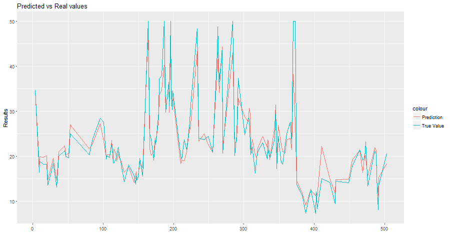
You can also plot your predicted values and see the output:
# Plot the predictions against real values
library(ggplot2)

plot_predictions = ggplot(prediction_output, aes(ID)) +
                    geom_line(aes(y = PREDICTION, colour = "Prediction")) +
                    geom_line(aes(y = REALVALUE, colour = "True Value")) +
                    xlab("") +
                    ylab("Results") +
                    ggtitle("Predicted vs Real values")
                    theme(legend.title=element_blank())

plot(plot_predictions)