R Regression Tutorial

In this tutorial you will learn how to do regression analysis in Exasol using a UDF written in R.

This tutorial uses database objects in the free public demo system hosted by Exasol. To get access to the public demo system, sign up here.

Introduction

In this tutorial you will learn how to perform a simple regression analysis in Exasol by displaying JSON data stored in a column as a table. You will create a user defined function (UDF) in the R programming language and use this on an already trained model with sample data.

The tutorial will demonstrate that there is no need to export data from Exasol to a different system to apply machine learning models. Everything can be done using UDFs directly within the Exasol database where the data is stored.

To follow the tutorial you should have basic R programming knowledge and a basic understanding of Exasol and of what UDFs are. The tutorial does not require a deep understanding of data science or machine learning methods.

Procedure

You can choose to write the R UDFs in your SQL client, or you can create them in an R development environment using the r-exasol package. The advantage of creating the UDFs in an R environment is that you can play around with dataframes in R and visualize the results in the IDE. Both methods are shown in the tutorial, and the result will be the same regardless of which method you choose.

About the data set

Imagine that you are planning a conference in Phoenix, AZ with a large number of attendees from all over the US. In this scenario, you may want to advise the attendees on which weekday will be the best for them to fly back in order to get a flight with minimum delay.

The data set used in this tutorial contains historical data on domestic flights in the US over a number of years, including information about delays. The public demo database already contains a random forest model trained on a sample from this data set, based on the airline, flight number, and day of the week. In the tutorial you will learn how to use this model to predict the delay for flights on specific weekdays.

R scripts must be compiled with Unix/Linux line endings (LF). If you are using an SQL client on Windows, you must set the linefeed to LF in the client before executing R scripts. To learn more, refer to the documentation for the respective client.

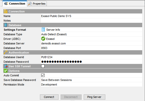
Step 1: Connect to the Exasol public demo system

# If needed, install devtools.
install.packages("devtools")

# Install package using devtools.
devtools::install_github("EXASOL/r-exasol")

# If needed, install and load these libraries.
library(exasol) # Exasol package
install.packages('RODBC')
library(RODBC) # ODBC database connectivity

exaconn <- dbConnect(
    drv = "exa", # EXAdriver object
    exahost = "demodb.exasol.com:8563", # host name or IP address of the database cluster
    uid = "<YOUR_USER>", # database username
    pwd = "<YOUR_PASSWORD>") # database password

odbcQuery(exaconn, "OPEN SCHEMA <YOUR_USERNAME>");

Step 2: Examine the data

To understand the data structure in our example, look at the FLIGHTS table in the FLIGHTS schema.

-- count the number of rows in the table
select count(*) from FLIGHTS.FLIGHTS;
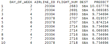
-- get a preview of the test data
select * from FLIGHTS.FLIGHTS LIMIT 10; 

# count the number of rows in the table
dbGetQuery(exaconn, "select count(*) from FLIGHTS.FLIGHTS")
# get a preview of the test data
dbGetQuery(exaconn, "select * from FLIGHTS.FLIGHTS LIMIT 10")

Step 3: Create an R UDF for flight delay prediction

When you have established a connection to the database and you understand the structure of the test data, the next step is to create a UDF to predict delays based on the data.

In this tutorial you will create a UDF called FLIGHTS_PRED_DEP_DELAY. The input parameters for this UDF are the columns that should be considered for delay prediction, which are the following:

• AIRLINE_ID (the airline ID)
• FLIGHT_NUM (the flight number)
• DAY_OF_WEEK (the day of week for the flight)

For every input, the UDF will output a line containing the input parameters plus the predicted delay. Instead of creating a SCALAR RETURNS function, we use a SET EMITS function here. This means that the function will not only get a single row as input but multiple rows at once. The GROUP BY statement determines the number of rows each instance of the UDF works on, more details will follow in the next section.

BucketFS

Exasol systems use a distributed file system called BucketFS. A BucketFS service contains buckets that can store files, and each bucket can have different access privileges. In your UDF you will use a model which is stored in a publically readable bucket in the demo system, which means that you do not have to define a password. The model will then be applied to data that is read into a data frame object.

-- open your own schema 
 OPEN SCHEMA <YOUR_USER_NAME>;

CREATE OR REPLACE R SET SCRIPT 
    "FLIGHTS_PRED_DEP_DELAY" ("DAY_OF_WEEK" DECIMAL(18,0), 
    "AIRLINE_ID" DECIMAL(18,0), 
    "FLIGHT_NUM" DECIMAL(18,0), 
    "DEST" CHAR(3) UTF8)
    EMITS (
        "AIRLINE_ID" DECIMAL(18,0), 
        "FLIGHT_NUM" DECIMAL(18,0), 
        "DAY_OF_WEEK" DECIMAL(18,0), 
        "DEST" VARCHAR(200000) UTF8, 
        "PREDICTED_DELAY_IN_MINUTES" DECIMAL(16,14))
    AS
        run <- function(ctx) {
            # load the required package
            require(randomForest)
            # load the flightModel from BucketFS and unserialize it for use
            f <- file("/buckets/bucketfs1/demo_flights/flightModel", open="r", raw=TRUE)
            m <- unserialize(f)
            # work on the data in chunks of 1000 elements
            repeat {
            if(!ctx$next_row(1000))
            break
            # load data into dataframe
            df <- data.frame(
            DAYOFWEEK = ctx$DAY_OF_WEEK,
            AIRLINE_ID = ctx$AIRLINE_ID,
            FLIGHTNUM = ctx$FLIGHT_NUM,
            DEST = ctx$DEST
            )
            # predict the delay and emit (create the result set)
            prediction <- predict(m, newdata = df)
            ctx$emit(df$AIRLINE_ID,df$FLIGHTNUM,df$DAYOFWEEK,df$DEST,prediction)
        }
    }
/                

PredictInExasolFinal <- exa.createScript(
    exaconn,
    "FLIGHTS_PRED_DEP_DELAY",
    function(ctx) {
    # load the required package
    require(randomForest)
    # load the flightModel from BucketFS and unserialize it for use
    f <- file("/buckets/bucketfs1/demo_flights/flightModel", open="r", raw=TRUE)
    m <- unserialize(f)
    # load the data in chunks and save it in a dataframe
    repeat {
    if(!ctx$next_row(1000))
    break
    # put data into dataframe
    df <- data.frame(
    DAYOFWEEK = ctx$DAY_OF_WEEK,
    AIRLINE_ID = ctx$AIRLINE_ID,
    FLIGHTNUM = ctx$FLIGHT_NUM,
    DEST = ctx$DEST
    )
    prediction <- predict(m, newdata = df)
    ctx$emit(df$AIRLINE_ID,df$FLIGHTNUM,df$DAYOFWEEK,df$DEST,prediction)
    }
    },
    # input arguments
    inArgs = c(
    "DAY_OF_WEEK DECIMAL(18,0)",
    "AIRLINE_ID DECIMAL(18,0)",
    "FLIGHT_NUM DECIMAL(18,0)",
    "DEST CHAR(3)"
    ),
    # output arguments
    outArgs = c(
    "DAY_OF_WEEK DECIMAL(18,0)",
    "AIRLINE_ID DECIMAL(18,0)",
    "FLIGHT_NUM DECIMAL(18,0)",
    "DEST VARCHAR(200000)",
    "PREDICT DOUBLE"
    ),
    # replace existing version (optional)
    replaceIfExists = TRUE
)

Step 4: Let the model predict

The next step is to create the view PRED_DELAY, which will enable access to the prediction data. The UDF is executed every time the PRED_DELAY view is queried. This means that if new rows are added the the FLIGHTS table, the view will work on the updated data when it is queried.

You want to run our UDF for each combination of airline id, flight number, day of the week, and destination. Additionally, you are only interested in flights departing from PHX. Therefore, you include a subselect to execute the UDF on the appropriate data set.

To execute the UDF in parallel, you will use a GROUP BY statement together with the IPROC() function, which returns a different number for each node in the cluster. The GROUP BY statement will start one process for each group. This means that GROUP BY IPROC() will start as many instances of the UDF as we have nodes.

CREATE OR REPLACE VIEW FLIGHTS_PRED_DELAY_PHX AS (
    WITH FLIGHTS_PRE_SELECTION AS (
        SELECT AIRLINE_ID,FLIGHT_NUM,DAY_OF_WEEK,DEST
        FROM FLIGHTS.FLIGHTS
        WHERE ORIGIN = 'PHX'
        GROUP BY AIRLINE_ID,FLIGHT_NUM,DAY_OF_WEEK,DEST
    )
    SELECT "FLIGHTS_PRED_DEP_DELAY" (DAY_OF_WEEK, AIRLINE_ID,FLIGHT_NUM,DEST)
    FROM FLIGHTS_PRE_SELECTION
    GROUP BY IPROC()

CREATE TABLE FLIGHT_PREDICTION_PERSISTED AS (
    SELECT * FROM FLIGHTS_PRED_DELAY_PHX
    );

odbcQuery(exaconn, "CREATE OR REPLACE TABLE FLIGHTS_PRE_SELECTION as select DAY_OF_WEEK,AIRLINE_ID,FLIGHT_NUM,DEST from FLIGHTS.FLIGHTS where ORIGIN = 'PHX' group by DAY_OF_WEEK,AIRLINE_ID,FLIGHT_NUM,DEST")

prediction_output = PredictInExasolFinal(
"DAY_OF_WEEK",
"AIRLINE_ID",
"FLIGHT_NUM",
"DEST",
table="FLIGHTS_PRE_SELECTION",
groupBy = "iproc()"
)

Step 5: Visualize the data

You can now visualize the data that you predicted with the UDF by connecting your favorite data visualization tool to Exasol. You can also create a visualization directly in R.

R environment visualization

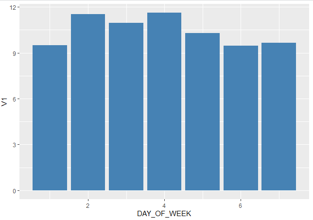
The following example draws a bar plot on mean of prediction values grouped by day of week.

install.packages("data.table")
    library(data.table)
    DT <- data.table(prediction_output)
    DT <- DT[, mean(PREDICT), by = DAY_OF_WEEK]
    DT
    install.packages("ggplot2")
    library(ggplot2)
    # Basic barplot
    p<-ggplot(data=DT, aes(x=DAY_OF_WEEK, y=V1)) +
    geom_bar(stat="identity", fill="steelblue")
    print(p)