Appropriate Data Types
- Choosing appropriate data types is a key factor during data modeling. It provides a good compression and avoids unnecessary type conversions or expression indexes.
- Keep formats short, do not use VARCHAR(2000000) or DECIMAL(32,X) if a smaller range is sufficient.
-
Prefer exact data types.
- Prefer DECIMAL over DOUBLE if possible. Double has a wider scale but is less efficient.
- Prefer CHAR(x) over VARCHAR(x) if the length of the strings is a known constant (CHAR is fixed size).
- Use identical types for same content: Avoid joining columns of different data types. For example, do not join an INT column with a VARCHAR column containing digits.
- See Exasol GitHub repository to learn more about appropriate data types.
Replication
To increase the speed of queries, the Exasol query optimizer replicates "small tables" of a query so that global joins become fast local joins. During query execution, all needed data from “small tables” are replicated in local DBRAM and data from all nodes is accessed locally. No communication is needed and access is very fast. Since the data resides in DBRAM, multiple queries that need the same data can share the replicated data.
The replication border sets the upper size limit for a "small table" that the query optimizer will consider replicating. The default replication border is 100,000 rows. This border can be increased. For example, if you have a star schema, consider increasing the replication border so that all your dimension tables are replicated.
-soft_replicationborder_in_numrows=<number_of_rows>.
The query optimizer may not replicate all tables that fit within the replication border. For example, modified tables that are not committed will not be considered by the query optimizer for replication even when the tables fit within the replication border.
Distribution Keys
Distribution key scenarios
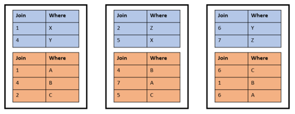
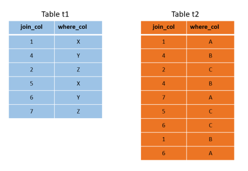
Any table whose size exceeds the replication border (large tables) is distributed on a row-by-row basis across all active nodes. Without specifying a distribution key, the distribution is random and uniform across all nodes. Setting a proper distribution key on join columns of the same data type converts global joins to local joins and improves performance. Take the following two tables as an example:

The tables are joined on the join_col and filtered on the where_col. Other columns are not displayed to keep the sketch small. Small tables like these are normally replicated, but for this example, we ignore that. A random distribution on a three node cluster may look like this:
If the tables are now joined on the join_col with the following statement, the random distribution is not optimal:
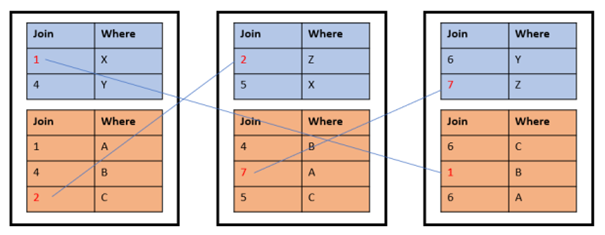
This is processed as a global join internally. It requires network communication between the nodes on behalf of the join because the highlighted rows don't find local join partners on the same node.
You can change the distribution of both tables using the following statements, allowing the system to recognize a match between join column and table distribution.
You can only set one distribution key per table.
Then the same query is processed internally as a local join:
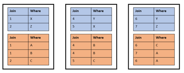
Every row finds a local join partner on the same node, so the network communication between the nodes on behalf of the join is not required. The performance with this local join is better than with the global join although it’s the same SELECT statement.
It’s a good idea to distribute on JOIN columns. However, it’s not good if you want to distribute columns that you use for filtering with WHERE conditions. If you distribute both tables on the where_col columns, the result will look like this:
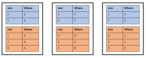
This distribution is worse than the initial random distribution. This causes global joins between the two tables and statements like <Any DQL or DML> WHERE t2.where_col='A'; utilize only one node (the first with this WHERE condition). This disables Exasol’s Massive Parallel Processing (MPP) functionality. This distribution leads to poor performance because all other nodes in the cluster are on standby while one node does all the work.
Exasol's resource management assumes uniform load across all nodes. Therefore, this distribution leads to resources being unused even when multiple simultaneous statements operate on different filter values (for example, nodes). The MPP relies on a near-uniform distribution of data across the nodes, so columns where few values dominate the table are usually bad candidates for distribution. Distributing by a combination of columns (see Distribution on multiple columns) may alleviate this problem.
Distribution on multiple columns
The ALTER TABLE (Distribution/Partitioning) statement allows distribution over multiple columns in a table. However, to take advantage of this, all those columns must be present in a join. Therefore, for most scenarios, distributing by a single column is appropriate. The requirement for a local join is that the distribution columns for both tables must be a subset of the columns involved in the join. Let's look at the following example. Imagine you have two tables defined with the following DDL:
CREATE TABLE T1 (
    X INT,
    Y INT,
    Z INT,
    DISTRIBUTE BY X
);

CREATE TABLE T2 (
    X INT,
    Y INT,
    Z INT,
    DISTRIBUTE BY X
);
Since these tables are both distributed by the column X, join conditions which include (but are not limited to) these columns will be local. This includes the following queries:
SELECT * FROM T1
JOIN T2 ON T1.X = T2.X;

SELECT * FROM T1
JOIN T2 ON T1.X = T2.X
AND T1.Y = T2.Y;

SELECT * FROM T1
JOIN T2 ON T1.X = T2.X
AND T1.Y = T2.Y
AND T1.Z = T2.Z;
Since the distribution keys (T1.X and T2.X) are included in each of the joins, the entire join is operated locally. Changing the distribution key to cover multiple columns will have a negative impact in this case. For example, let's distribute the tables now by columns X and Y:
Now, only the second and third examples will have local joins. A simple join on T1.X = T2.X will be a global join because the distribution keys are no longer a subset of the join conditions.
Check how a new distribution key distributes rows
Let's consider a scenario where you plan to change the distribution key to use column aa_00 and you want to see how it is going to distribute rows. This is a type of check that allows you to see the distribution before you implement the distribution key.
Run the following statement to check the distribution of the new distribution key.
SELECT value2proc(aa_000) as Node_Number, round(count(*) / sum(count(*)) over() * 100 ,2) as Percentage
from <table name>
group by 1;
If the distribution is very uneven or skewed, it is not recommended to implement the new distribution key.
Conclusion:
- Do: Distribute on JOIN columns to improve performance by converting global joins to local joins.
- Do: Pick the smallest viable set of columns that will be part of all your most frequent or expensive joins as distribution key.
- Don't: Distribute on WHERE columns, which leads to global joins and disables the MPP functionality, both causing poor performance.
- Don't: Add unneeded columns to a distribution key.
Avoid ORDER BY
Views are usually treated like tables by end users who aren't aware of an ORDER BY clause being part for the view’s query. This means that clause is superfluous and slows down the view performance. Similarly, ORDER BY clauses in sub-queries will slow down query performance and cause materialization which may not be required. There should be only one ORDER BY clause (if any) at the end of an SQL statement.
In some cases, using an ORDER BY FALSE statement to materialize a sub-select may actually improve performance. For more information, see Enforcing Materializations with ORDER BY FALSE.
Manual Index Creation
Exasol creates and maintains required indexes automatically. It is not recommended to interfere in this. For more information about how indexes work, see Indexes.
Use Surrogate Keys
Joins on VARCHAR and DATE/TIMESTAMP columns are expensive compared to joins on DECIMAL columns.
Joins on multiple columns generate multi-column indexes which require more space and effort to maintain internally compared to single column indexes.
Use instead surrogate keys to avoid above problems.
Favor UNION ALL
The difference between UNION and UNION ALL is that UNION eliminates duplicates, thereby sorting the two sets. This means UNION is more expensive than UNION ALL, so in cases where it is known that no duplicates can occur or when duplicates are acceptable, UNION ALL should be used instead of UNION.
Partitioning
If tables are too large respectively too many to fit completely into the node’s memory, partitioning large tables can help improve performance. Take these two tables as example:
Say t2 is too large to fit in memory and may get partitioned therefore.
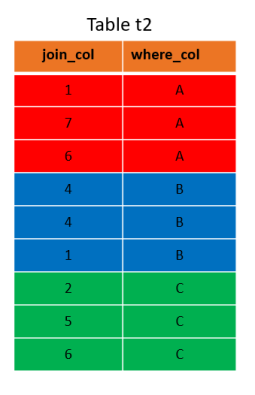
In contrast to distribution, partitioning should be done on columns that are used for filtering:
ALTER TABLE t2 PARTITION BY where_col;
Now without taking distribution into account (on a one-node cluster), the table t2 looks like this:
Partitioning changes the way the table is physically stored on disk. It may take much time to complete such an ALTER TABLE (Distribution/Partitioning) command with large tables.
A statement like SELECT * FROM t2 WHERE where_col=’A’; would have to load only the red part of the table into memory. Should the two tables reside on a three-node cluster with distribution on the join_col columns and the table t2 partitioned on the where_col column, they look like this:
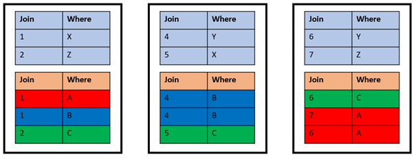
Again, this means that each node has to load a smaller portion of the table into memory if statements are executed that filter on the where_col column while joins on the join_col column are still local joins.
EXA_(USER|ALL|DBA)_TABLES (see Metadata System Tables) shows both the distribution key and the partition key if any.
Exasol will automatically create an appropriate number of partitions.
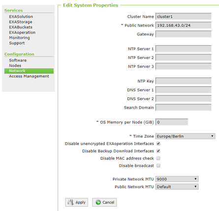
Use Jumbo Frames
The maximum transmission unit (MTU) can be set for the private and public networks in EXAoperation. Exasol data blocks have a minimum size of 4kB which does not fit into the default MTU size of 1500 bytes. For best performance we recommend using Jumbo Frames (MTU size of 9000 bytes). All network components must then be enabled to use MTU 9000. MTU 9000 must also be enabled in the license server.
Jumbo Frames are not supported with GCP.
Database Monitoring
The tables in the Statistical System Tables schema can be used to monitor the health of the database. They come with detailed values for the last 24 hours and aggregated values on an hourly, daily and monthly basis: EXA_DB_SIZE*, EXA_MONITOR*, EXA_SQL* and EXA_USAGE*. Other important tables to monitor are EXA_DBA_TRANSACTION_CONFLICTS and EXA_SYSTEM_EVENTS. The meta view EXA_SYSCAT lists all these tables together with a description.
CPU Utilization
A high CPU utilization is normal for a healthy system. Low CPU utilization (on a busy system) is an indicator that a bottleneck exists somewhere else. CPU_MAX from EXA_MONITOR_DAILY should be normally above 85% therefore.
TEMP Utilization
Analytical queries often consume a lot of memory for sort operations. The EXA_MONITOR* tables should be monitored to confirm that the total TEMP memory consumption is below 20% of the total available database RAM, while the EXA_SQL* and EXA_*_SESSIONS tables should be monitored to confirm that a single query doesn’t consume more than 10% of available database memory.
RAM Recommendation
Exasol performs well with parallel in-memory processing analytical queries. This requires sufficient memory availability. The EXA_DB_SIZE* tables have RECOMMENDED_DB_RAM_SIZE where the system reports if it would be beneficial to add more RAM to the data nodes.
Avoid the USING Syntax
The use of the USING syntax in queries containing multiple joins leads to an inefficient execution and high amount of heap memory usage by the SQL processes.
Example
In the above example, USING(id) is not just syntactic sugar for ON T1.id = T2.id. The database has to decide the values for the columns that appear in both the tables. For example, when T1.name has a NULL value, and T2.name is different from NULL, then the value of the output column name will be T2.name. This effort increases exponentially on the number of joins.
Instead, you can use the following statement for a better performance.