The intended audience for this tutorial is assumed to have a basic understanding of Exasol, in particular, user-defined functions (UDFs) and basic Python programming knowledge. The demonstration does not require a deep understanding of data science or machine learning methods. This tutorial serves the purpose of trying out user-defined functions (UDFs) on an available machine learning model with a test dataset.
The tutorials in this section are designed to work with the public demo system hosted by Exasol. If you have not already done so, sign up here to get access to the public demo system.
Model Testing with UDFs
Developing a typical machine learning model consists of multiple steps. First, you load the data, normalize the measures if necessary, build a model, train it, refine the parameters, and evaluate the performance. In order to simplify the process for this demo, we assume that we have already developed an adequate model that predicts truck failures and trained it accordingly. We will focus on the last steps, which is, running the model on the test data and evaluating its performance (steps 3 and 4 in the image below).
If you are interested in a full end-to-end demonstration of how the machine learning techniques can be directly applied in Exasol, refer to our Data Science GitHub repository.
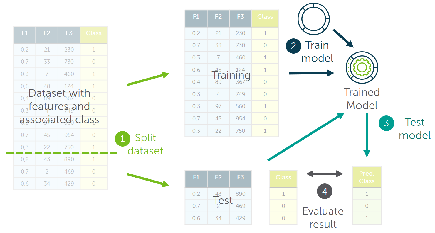
The result of the demo can be achieved with two different approaches, either by writing the UDFs in a SQL client or creating them directly out of a Python environment with the help of the pyexasol package. Both approaches will give us the same results in the end, the advantage of the latter one is that it allows you to play around with dataframes inside Python and lets you visualize results more easily. Both approaches will be displayed side by side in the tutorial and in the below sections so that you can choose your preferred one.
The Dataset: Predicting Truck Failures
We use real-world data provided by the truck manufacturer Scania to predict if truck failures are related to the failure of a specific component or not. The data is publicly available in the IDA 2016 Challenge dataset from the Industrial Challenge at the 15th International Symposium on Intelligent Data Analysis (IDA) in 2016. The purpose of the challenge was to predict, which failures were related to a specific component of a truck's air pressure system (APS) as opposed to failures unrelated to the APS.
In the process, we demonstrate that there is no need to export data from Exasol to a different system for training and testing machine learning models. Everything can be done using UDFs directly inside Exasol where the data is stored.
Procedure
For this demo, we will use a dataset on the publicly available Exasol demo system. If you haven't already, sign up for an account on this page. The schema we are working with is called "IDA". It contains multiple tables filled with training and test data.
Step 1: Connect to the Exasol Demo Database
As a first step, we will create a connection to the system and get familiar with the table structures. The following table provides you with the details on connecting to a database (using an SQL client) and Python environment.
SQL Client
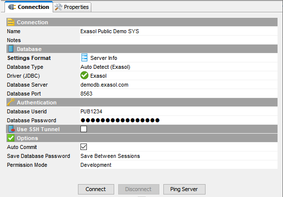
To connect to the system, you can use the SQL Client of your choice. Exasol recommends DbVisualizer in the Pro version, an open source alternative is the tool DBeaver. Enter the credentials you received by email.
Python Environment
For this demo, we use a Jupyter notebook running with Python 3.6.
To connect to Exasol, install the pyexasol package in your local Python environment. Depending on your package manager, you can either use
- pip install pyexasol[pandas] or
- conda install -c conda-forge pyexasol
If you're running inside a Jupyter notebook, add an exclamation mark before the statement.
Once you have installed pyexasol, we can start writing our script by specifying the connection details for the Exasol demo system that we will use later on.
Replace username and password with the credentials you received through email. Replace the schema name with your username in order to create the UDFs in your own schema.
EXASOL_HOST = "demodb.exasol.com:8563"
EXASOL_USER = "<YOUR_USER_NAME>"
EXASOL_PASSWORD = "<YOUR_PASSWORD>"
SCHEMA_NAME ="<YOUR_USER_NAME>"
With the following statement, we test the connectivity to the database:
import pyexasol
import textwrap

# Create Exasol connection
C = pyexasol.connect(dsn=EXASOL_HOST, user=EXASOL_USER, password=EXASOL_PASSWORD, compression=True)
# Test the connection
stmt = C.execute("SELECT 42 from DUAL")
print(stmt.fetchone()[0])
Now that the connection is opened, we can move on to the next step - Examine the data.
Step 2: Examine the Data
Before applying our model, we will get an understanding of the data structure by having a quick look at the relevant table in the IDA schema. As we will use an already trained model, we will only need the test data in a normalized format. This is stored in the table IDA_TEST_TRANSFORMED.
SQL Client
-- Examine the data:
-- how many rows does the table hold?
select count(*) from IDA.IDA_TEST_TRANSFORMED;

-- what does the data look like?
select * from IDA.IDA_TEST_TRANSFORMED LIMIT 10; -- get a preview of the test data
Python Environment
# Examine the data:
# How many rows does the table hold?
stmt = C.execute("select count(*) from IDA.IDA_TEST_TRANSFORMED")
print(stmt.fetchone()[0])
# How does the data look like?
# Get a preview of the test data
df = C.export_to_pandas("select * from IDA.IDA_TEST_TRANSFORMED LIMIT 5")
print(df.head())
Now that we've got an impression of the data, we will move on to the next step of preparing our environment for the creation of UDFs.
Step 3: Preparing the Environment
Exasol ships with a default language container for Python 3 that can be used to run Python UDFs out of the box in the database. This language container includes some commonly used data science modules. If you need further libraries not included in the default container or you want to use another version of Python, Exasol allows you to create your own script language containers including these. That way, you can create a custom UDF environment tailored to your needs. Refer to the Exasol Script Language GitHub Repository for instructions.
Additionally, Exasol has a distributed file system called BucketFS. The demo system is equipped with the bucket that includes our model (Model: classifier3.pkl). In the following step we will also define the details for accessing the content in this bucket.

BucketFS Service: bucketfs1
BucketFS Bucket:
demo_ida
SQL Client
In the below commands, replace <YOUR_USER_NAME> with your username and run the commands.
The following command will open your own schema on the demo system.
NOTE: Please note that schema is only set for the current session. Therefore, if you reconnect to the system, you have to execute this statement again.
-- Open your own schema, we will create our scripts in this schema later on
open schema <YOUR_USER_NAME>;
Python Environment
We define a few variables that contain information about the information about where to find the model that we want to test in the BucketFS.
EXASOL_BUCKETFS_SERVICE = "bucketfs1"
EXASOL_BUCKETFS_BUCKET = "demo_ida"
EXASOL_BUCKETFS_PATH = f"/buckets/{EXASOL_BUCKETFS_SERVICE}/{EXASOL_BUCKETFS_BUCKET}" # Filesystem-Path to the read-only mounted BucketFS inside the running UDF Container

EXASOL_BUCKETFS_USE_HTTPS = True

model_file = "classifier3.pkl"
The following command will open your own schema on the demo system.
NOTE: Please note that schema is only set for the current session. Therefore, if you reconnect to the system, you have to execute this statement again.
# Create Exasol connection
C = pyexasol.connect(dsn=EXASOL_HOST, user=EXASOL_USER, password=EXASOL_PASSWORD, compression=True)

# Open your own schema
C.execute(f"OPEN SCHEMA {SCHEMA_NAME}")
Step 4: Creating a Script to Test the Model
In this step we will create a Python UDF called IDA_TEST_MODEL, which will be used to predict results for the test data (i.e., whether a failure is an APS failure or not) in the next step. Therefore, the input parameters for the UDF are all the columns that should be considered for the failure prediction. Based on these, the UDF will emit results, that are the predicted classes (first column) joined to the transformed test data. By joining the predicted class labels to the test data, we ensure that the predicted and real class labels remain properly ordered / linked for evaluation as we don't have a smaller set of columns that uniquely identifies each row.
As we have 170 measures to take into account, manually typing the list of input and output parameters would be quite some work. Therefore, we use the system tables containing the column names and column types to generate these for us.
SQL Client
In this case, we use a small helper statement to do the work for us. The output of this statement is a list of all the columns which can copy into our script at the right places before creating it.
SELECT group_concat(column_name || ' ' || column_type ORDER BY column_ordinal_position) AS input_cols
        FROM    exa_all_columns c
        WHERE   column_schema = 'IDA'
        AND     column_table = 'IDA_TEST_TRANSFORMED';
Copy the script below in your SQL Client. Next, execute the above statement and copy the output to the script below at the two places where it says <replace with your list>. Afterward, execute it to create the script.
If you are using DbVisualizer, you have to disable Parameterized SQL before executing a script containing '&' - Symbols. Otherwise, the SQL client requests you to enter values for the parameters. To disable Parameterized SQL, navigate to SQL Commander --> SQL Commander Options and uncheck Parameterized SQL option.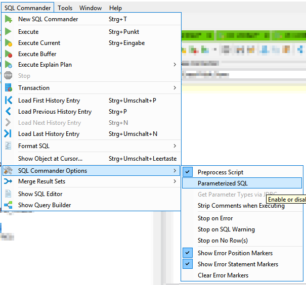
--/
CREATE OR REPLACE PYTHON3 SET SCRIPT IDA_TEST_MODEL(CLASSIFIER_PATH VARCHAR(200),<replace with your list>
)
 EMITS (CLASS_PRED DECIMAL,<replace with your list>
) AS

import pandas as pd
from sklearn.externals import joblib

# Test classifier
def test(X, class_col_name, model_path=None):
    # Convert columns to numeric data types
    X = X.apply(pd.to_numeric)

    X_data = X.loc[:, X.columns != class_col_name]

    # Load model from EXABucket
    clf = joblib.load(model_path)

    # Predict classes of test data
    return clf.predict(X_data)

def run(ctx):
    # Input argument
    num_non_data_cols = 1
    classifier_path = ctx.CLASSIFIER_PATH

    df = ctx.get_dataframe(num_rows='all', start_col=num_non_data_cols)

    # Test the classifier
    y_pred = test(df, class_col_name='CLASS', model_path=classifier_path)

    # Add class predictions as first column of test DataFrame
    df_pred = (pd.DataFrame(y_pred, columns=['CLASS_PRED'])).join(df)

    # Convert columns to numeric data types
    df_pred = df_pred.apply(pd.to_numeric)

    # Output data
    ctx.emit(df_pred)
/
Python Environment
We define a few variables that contain information about the information about where to find the model that we want to test in the BucketFS.
# Read one line of the dataset to get the structure
df = C.export_to_pandas("SELECT * FROM IDA.IDA_TEST_TRANSFORMED LIMIT 1")

# Create tables for data
column_names = list(df.columns)

###column_types = ["VARCHAR(3)"] + ["DECIMAL(18,2)"] * (len(column_names))
###column_desc = [" ".join(t) for t in zip(column_names, column_types)]

# Numeric data
column_types = ["INT"] + ["DOUBLE"] * (len(column_names) - 1)
column_desc = [" ".join(t) for t in zip(column_names, column_types)]


# Create script output column descriptions
# One class label, numeric data
out_column_types = ["INT"] * 2 + ["DOUBLE"] * (len(column_names))
out_column_desc = [" ".join(t) for t in zip(["class_pred"] + column_names, out_column_types)]

# Create script to test the model
sql = textwrap.dedent(f"""\
CREATE OR REPLACE PYTHON3 SET SCRIPT IDA_TEST_MODEL(CLASSIFIER_PATH VARCHAR(200), {", ".join(column_desc)}
)
EMITS ({", ".join(out_column_desc)}) AS
import pandas as pd
from sklearn.externals import joblib


# Test classifier
def test(X, class_col_name, model_path=None):
    # Convert columns to numeric data types
    X = X.apply(pd.to_numeric)

    X_data = X.loc[:, X.columns != class_col_name]

    # Load model from EXABucket
    clf = joblib.load(model_path)

    # Predict classes of test data
    return clf.predict(X_data)

def run(ctx):
    # Input argument
    num_non_data_cols = 1
    classifier_path = ctx.CLASSIFIER_PATH

    df = ctx.get_dataframe(num_rows='all', start_col=num_non_data_cols)

    # Test the classifier
    y_pred = test(df, class_col_name='CLASS', model_path=classifier_path)

    # Add class predictions as first column of test DataFrame
    df_pred = (pd.DataFrame(y_pred, columns=['CLASS_PRED'])).join(df)

    # Convert columns to numeric data types
    df_pred = df_pred.apply(pd.to_numeric)

    # Output data
    ctx.emit(df_pred)
/
""")

C.execute(sql)
Step 5: Let the Model Predict
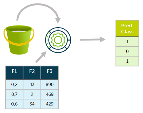
We are now prepared to run the data science model for prediction and evaluation on the data. We will run the prediction by executing the script we just created and store the results in the table TEST_PREDICTIONS.
The UDF TEST_MODEL takes the path to our model and all the input columns as input parameters. So the first parameter we hand over to the UDF is the path to our model in BucketFS. The following input parameters are the columns of our table with test data.
SQL Client
As mentioned in the step before, we need all the columns as input parameters for our script and do not want to type them manually. Therefore, we use the following statement to generate the column list for us.
SELECT group_concat(column_name ORDER BY column_ordinal_position) AS input_cols
        FROM    exa_all_columns c
        WHERE   column_schema = 'IDA'
        AND     column_table = 'IDA_TEST_TRANSFORMED';
Copy the statement below in your SQL Client. Then, execute the statement above and copy the output in the script below where it says <replace with your list>. Afterward, execute the statement to create the table TEST_PREDICTIONS.
-- Create a new table in your own schema
CREATE OR REPLACE TABLE IDA_TEST_PREDICTIONS AS
 SELECT IDA_TEST_MODEL('/buckets/bucketfs1/demo_ida/classifier3.pkl',<replace with your list>)
FROM IDA.IDA_TEST_TRANSFORMED;
This table will be used to evaluate our results. Here's a short preview of our predictions table created by running the script.

Step 6: Evaluating the Model
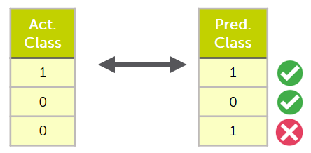
In the resulting table IDA_TEST_PREDICTIONS, we now have a column with the prediction made by our model CLASS_PRED and the actual label as the ground of truth in the column CLASS. We will compare these two columns in the next step to evaluate how well our model performed. We use a cost function which we call ida_cost() as a performance metric, which implements the cost function specified in the problem description. Additionally, we create a confusion matrix that displays how the instances were classified.
SQL Client
Create the following:
--/
CREATE OR REPLACE PYTHON3 SET SCRIPT IDA_EVALUATE_RESULTS(CLASS_PRED double, CLASS double)
EMITS (RESULTS varchar(200),PREDICTED_NEG double, PREDICTED_POS double, TOTAL_COSTS double) AS

from sklearn.metrics import confusion_matrix
import pandas as pd
import pyexasol
import numpy as np

# Define cost function from the problem description
def ida_cost(y, y_pred):
    false_preds = y - y_pred
    num_false_pos = (false_preds < 0).sum()
    num_false_neg = (false_preds > 0).sum()
    return 10 * num_false_pos + 500 * num_false_neg

def evaluate(df):
    y_pred = df.loc[:, 'CLASS_PRED']
    y = df.loc[:, 'CLASS']

    # Examine the results
    confusion_mat = confusion_matrix(y, y_pred)
    confusion_matrix_df = pd.DataFrame(confusion_mat, columns=['predicted neg', 'predicted pos'])

    matrix = np.array(['actual_neg','actual_pos'])
    confusion_matrix_df = pd.DataFrame(confusion_mat,
    columns=['predicted neg', 'predicted pos'])
    confusion_matrix_df["results"] = matrix
    df = confusion_matrix_df[['results','predicted neg','predicted pos']]
    df['Total costs'] = None
    total_cost = ida_cost(y,y_pred)
    df.loc[df.index.max() + 1] = ['Total costs',None,None,total_cost]

    return df

def run(ctx):
    df = ctx.get_dataframe(num_rows='all')
    results = evaluate(df)
    ctx.emit(results)
/
Python Environment
from sklearn.metrics import confusion_matrix
import pandas as pd

# Define cost function from the problem description
def ida_cost(y, y_pred):
    false_preds = y - y_pred
    num_false_pos = (false_preds < 0).sum()
    num_false_neg = (false_preds > 0).sum()
    return 10 * num_false_pos + 500 * num_false_neg

# Get predicted and real class labels
test_preds = C.export_to_pandas("SELECT CLASS_PRED, CLASS FROM IDA_TEST_PREDICTIONS")


y_pred = test_preds.loc[:, 'CLASS_PRED']
y = test_preds.loc[:, 'CLASS']

# Examine the results
confusion_mat = confusion_matrix(y, y_pred)
confusion_matrix_df = pd.DataFrame(confusion_mat,
                                   index=['actual neg', 'actual pos'],
                                   columns=['predicted neg', 'predicted pos'])

print("Confusion Matrix:\n", confusion_matrix_df)
print("\nTotal Cost:", ida_cost(y, y_pred),"\n")
Step 7: Confusion Matrix
After running the above evaluation script, the following results should be displayed.
| Predicted Neg | Predicted Pos | |
| Actual Neg | 14866 | 759 |
| Actual Pos | 6 | 369 |
| Total Cost: 10590 | ||
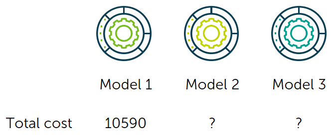
With the confusion matrix and the total cost, we can now compare our model to others.
Now you have seen how to evaluate a model using UDFs. If you are interested in the creation of a machine learning model in the database, refer to the Jupyter Notebook section in our Data Science GitHub repository.
